Some new or forgotten knowledge points

一些新的和遗忘的知识点

# Strain rate 应变速率 /deformation rate 变形速率

根据论文中的定义，
$u_x=\frac{1}{A}\oint u \text{d}y \approx \frac{1}{A} \sum_{i=1}^{n} \frac{1}{2}\left ( u_{i+1}+u_i\right )\left ( y_{i+1}-y_i\right )$,
$u_y=-\frac{1}{A}\oint u \text{d}x$,
$v_x=\frac{1}{A}\oint v \text{d}y$,
$v_y=-\frac{1}{A}\oint v \text{d}x$,

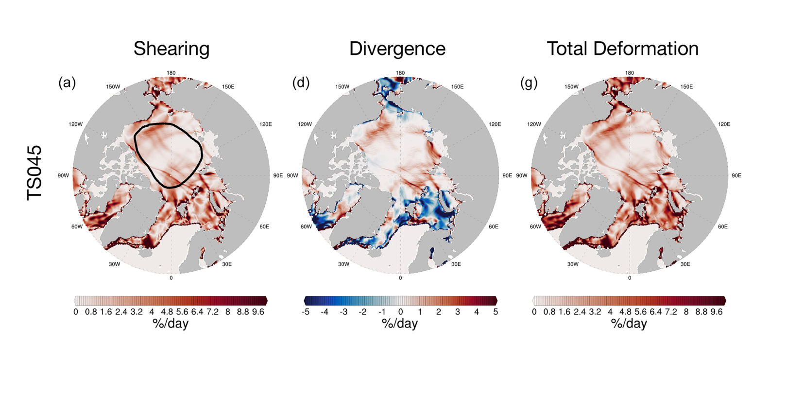
剪切率 $\dot{\varepsilon}_{\textrm{shear}}=\sqrt{\left ( u_{x}-v_{y}\right )^2+\left ( u_{y}+v_{x}\right )^2}$,
散度率 $\dot{\varepsilon }_{\textrm{div}} = u_x+v_y$,
总应变率 $\dot{\varepsilon }_{\textrm{tot}}=\sqrt{\dot{\varepsilon }_{\textrm{shear}}^{2}+\dot{\varepsilon }_{\textrm{div}}^{2}}$。

Strain rate is the rate of deformation caused by strain in a material within a corresponding time. This gauges the rate where distances of materials change within a respective period of time.

# B-grid

CSIM uses a generalized orthogonal B-grid, where tracer quantities are located at the center of the grid cells, and velocities are located at the corners. The internal ice stress tensor takes four different values within a grid cell. Tracer quantities in the ice model include ice and snow area, volume, energy and temperature. The grid comprised of the center points of the grid cells is referred to as the “T grid”. The “U grid” is comprised of the ponts at the northeast corner of the corresponding cell on the T grid. Quantities that are defined on the U grid include ice and ocean dynamics variables.

计算应变速率所需要的速度是定义在 U grid 上的，也就是每个 cell 的右上（东北）角。

参考页面

# 概率分布

# 随机变量的定义

设$\left ( \Omega,\mathscr{F},P\right )$ 为概率空间，$\xi =\xi(\omega )$ 为$\Omega$ 上定义的实值函数。如果有

$\left \{ \omega:\xi(\omega) < x \right \} \in \mathscr{F}, \forall x \in \mathbb{R},$

则称$\xi(\omega)$ 为随机变量。

时常将$\xi(\omega), \left \{ \omega:\xi(\omega) < x \right \}$ 等简写为$\xi, \{\xi < x\}$。

# 分布函数

$F(x)=\mathbf{F} \{(-\infty,x)\} =P\{\xi < x\}, x \in \mathbb{R}$ 为随机变量 $\xi$ 的分布函数。且称 $\xi$ 服从 $F(x)$，记为$\xi \sim F(x)$。有时也用 $F_\xi(x)$ 表明是 $\xi$ 的分布函数。

在论文中称其为 Cumulative Density Functions（累积密度函数），定义为

$cdf(x)=\mathbf{F} \{(x,\infty)\} =P\{\xi > x\}, x \in \mathbb{R}$，记为 $P(x) \sim cdf(x)$。

# 密度函数

若存在函数$p(x)$，满足 $p(x)>0, \int_{\mathbb{R}} p(x) \text{d}x=1$,
使得 $F(x)=\int_{-\infty}^x p(t) \text{d}t, x\in \mathbb{R}$，
则称 $\xi$（及其概率分布）为连续性的，$p(x)$ 为密度函数，简称密度。
论文中成为 Probability Density Functions（概率密度函数）。

# 期望

离散型：对概率分布 $p_i=P\{\xi=x_i\}, i=1,2,...$。若 $\sum_i |x_i|p_i < +\infty$，则

$E(\xi)=\sum_i x_i p_i$ 为数学期望。
连续性：若 $\int_{-\infty}^{+\infty} |x|p(x)\text{d}x < +\infty$，则
$E(\xi)=\int_{-\infty}^{+\infty} xp(x)\text{d}x$ 为数学期望。

# 方差

$D(\xi)=E (\left [ \xi-E(\xi) \right ]^2) = \int_{-\infty}^{+\infty} \left[ x-E(\xi) \right]^2 p(x)\text{d}x$，
$D(\xi)= E(\xi^2)-\left[ E(\xi)\right]^2$。

# 矩

k 阶原点矩（the $k^{\text{th}}$ moments）：$E(\xi^k)$
k 阶中心矩（the $k^{\text{th}}$ central moments）：$E(\left[ \xi-E(\xi) \right]^k)$
样本统计 k 阶原点矩: $\frac{1}{N}\sum_{i=1}^{N} x_i^k$

参考页面